My brother, Lucas, was in town and he told me about a recent video covering a beltless CVT transmission. As a student who created a CVT for his senior design project, he was very excited to share the video with me.

Inspiration

https://www.youtube.com/watch?v=mWJHI7UHuys

Setup

What we are solving for is essentially a classical four bar linkage which has been demonstrated by radcli14 before but ours has a little twist to it. What makes this special is the second bar ($B$) is not a fixed length but instead a dependant variable of the input angle. Also, the angle of the third bar ($\theta_3$) is a function of the angle of bar $B$.

I am using Sympy to perform the calculations and Manim for the animation

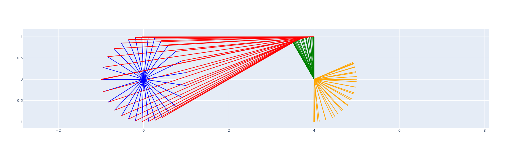
The red line is our “chain”. Bar $A$ is not rotating at a constant velocity. This is because it the “input” is to be attached to an elliptical gear which meshed with another gear about point $A$ causing $\theta_1$ to change in speed depending on the angle of the lobe at the given point in time. The reason why we used an elliptical gear will be discussed later on.

There are two guides that helped me with the rest of the setup:

• https://gist.github.com/radcli14/1e5923cc3927debc755aada7f40eb22c
• https://moorepants.github.io/learn-multibody-dynamics/configuration.html

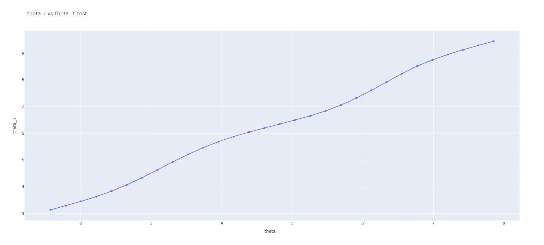
Analysis

Elliptical Gear

We will use $\theta_i$ and $\omega_i$ as the input angle and velocity for the first lobed gear and have $\theta_1$ and $\omega_1$ represent the second lobed gear as a function of the input one.

$\displaystyle r_{i} \dot{\theta}_{i} = r_{1} \dot{\theta}_{1}$

re-arranging for $\dot{\theta}_{1}$

$\dot{\theta}_{1}\, = \,\frac{\sqrt{- e^{2} \cos^{2}{\left(\theta_{1} \right)} + 1} \dot{\theta}_{i}}{\sqrt{- e^{2} \cos^{2}{\left(\theta_{i} \right)} + 1}}$

solving this with an ODE solver results in the expected non-constant rotation between the two gears

Kinematics

Rotation matrix for each frame

$\mathbf{R}_A \, = \,\left[\begin{matrix}\cos{\left(\theta_{1} \right)} & \sin{\left(\theta_{1} \right)} & 0\\- \sin{\left(\theta_{1} \right)} & \cos{\left(\theta_{1} \right)} & 0\\0 & 0 & 1\end{matrix}\right]$

$\mathbf{R}_B \, = \,\left[\begin{matrix}\cos{\left(\theta_{2} \right)} & \sin{\left(\theta_{2} \right)} & 0\\- \sin{\left(\theta_{2} \right)} & \cos{\left(\theta_{2} \right)} & 0\\0 & 0 & 1\end{matrix}\right]$

$\mathbf{R}_C \, = \,\left[\begin{matrix}\sin{\left(\theta_{2} \right)} & - \cos{\left(\theta_{2} \right)} & 0\\\cos{\left(\theta_{2} \right)} & \sin{\left(\theta_{2} \right)} & 0\\0 & 0 & 1\end{matrix}\right]$

Angular rate for each frame

$\mathbf{\omega}_A \, = \, \omega_{1}\mathbf{\hat{n}_z}$

$\mathbf{\omega}_B \, = \, \omega_{2}\mathbf{\hat{n}_z}$

$\mathbf{\omega}_C \, = \, \omega_{2}\mathbf{\hat{n}_z}$

while we are at it, create the roation matrix and angular for the output frame. This is entirely dependant on the kinematic system.

$\mathbf{R}_{OF} \, = \,\left[\begin{matrix}- \sin{\left(\theta_{2} + \frac{l_{b}}{l_{c}} \right)} & \cos{\left(\theta_{2} + \frac{l_{b}}{l_{c}} \right)} & 0\\- \cos{\left(\theta_{2} + \frac{l_{b}}{l_{c}} \right)} & - \sin{\left(\theta_{2} + \frac{l_{b}}{l_{c}} \right)} & 0\\0 & 0 & 1\end{matrix}\right]$

$\mathbf{\omega}_{OF} \, = \, (\omega_{2} + \frac{\dot{l_b}}{l_{c}})\mathbf{\hat{n}_z}$

Constraints

Positions constraint equation

$l_{c}\mathbf{\hat{c}_x} + l_{b}\mathbf{\hat{b}_x} + l_{a}\mathbf{\hat{a}_x} - l_{n}\mathbf{\hat{n}_x} \, = \, 0$

Positions constraint with respect to inertial frame

$\left[\begin{matrix}l_{a} \cos{\left(\theta_{1} \right)} + l_{c} \sin{\left(\theta_{2} \right)} - l_{n} + l_{b} \cos{\left(\theta_{2} \right)}\\l_{a} \sin{\left(\theta_{1} \right)} - l_{c} \cos{\left(\theta_{2} \right)} + l_{b} \sin{\left(\theta_{2} \right)}\end{matrix}\right]$

Velocity constraint

$l_{c} \omega_{2}\mathbf{\hat{c}_y} + \dot{l}_{b}\mathbf{\hat{b}_x} + l_{b} \omega_{2}\mathbf{\hat{b}_y} + l_{a} \omega_{1}\mathbf{\hat{a}_y} \, = \, 0$

Velocity constraint with respect to inertial frame

$\left[\begin{matrix}- l_{a} \omega_{1} \sin{\left(\theta_{1} \right)} + l_{c} \omega_{2} \cos{\left(\theta_{2} \right)} + \dot{l_b} \cos{\left(\theta_{2} \right)} - l_{b} \omega_{2} \sin{\left(\theta_{2} \right)}\\l_{a} \omega_{1} \cos{\left(\theta_{1} \right)} + l_{c} \omega_{2} \sin{\left(\theta_{2} \right)} + \dot{l_b} \sin{\left(\theta_{2} \right)} + l_{b} \omega_{2} \cos{\left(\theta_{2} \right)}\end{matrix}\right]$

Our velocity constraint is not very useful at the moment since it is composed of some dependant variables we do not know the values for. The variables it is composed of are

$\displaystyle \left\{\dot{l_b}, l_{b}, \omega_{1}, \omega_{2}, \theta_{1}, \theta_{2}\right\}$

We can see that the expressions are linear in $\omega_1$, $\omega_2$ and $\dot{l}_b$. If we select $\omega_{2}$ and $\dot{l_b}$ to be dependent, we can solve the linear system $\mathbf{A}\bar{x}=\bar{b}$ for those variables using the technique shown in Solving Linear Systems. First we define a column vector holding the dependent variables:

Our velocity constraint is

$f = \displaystyle \left[\begin{matrix}- l_{a} \omega_{1} \sin{\left(\theta_{1} \right)} + l_{c} \omega_{2} \cos{\left(\theta_{2} \right)} + \dot{l_b} \cos{\left(\theta_{2} \right)} - l_{b} \omega_{2} \sin{\left(\theta_{2} \right)}\\l_{a} \omega_{1} \cos{\left(\theta_{1} \right)} + l_{c} \omega_{2} \sin{\left(\theta_{2} \right)} + \dot{l_b} \sin{\left(\theta_{2} \right)} + l_{b} \omega_{2} \cos{\left(\theta_{2} \right)}\end{matrix}\right]$

Taking the jacobian of it with respect to $\omega_{2}$ and $\dot{l_b}$

$\mathbf{A} = \mathbf{J}_f(\omega_{2}, \dot{l_b}) = \displaystyle \left[\begin{matrix}l_{c} \cos{\left(\theta_{2} \right)} - l_{b} \sin{\left(\theta_{2} \right)} & \cos{\left(\theta_{2} \right)}\\l_{c} \sin{\left(\theta_{2} \right)} + l_{b} \cos{\left(\theta_{2} \right)} & \sin{\left(\theta_{2} \right)}\end{matrix}\right]$

Then find the terms not linear in the dependent variables:

$\bar{b} = \displaystyle \left[\begin{matrix}l_{a} \omega_{1} \sin{\left(\theta_{1} \right)}\\- l_{a} \omega_{1} \cos{\left(\theta_{1} \right)}\end{matrix}\right]$

results in

$\bar{x} = \displaystyle \left[\begin{matrix}\frac{l_{a} \omega_{1} \cos{\left(\theta_{1} - \theta_{2} \right)}}{l_{b}}\\- \frac{l_{a} \left(l_{c} \cos{\left(\theta_{1} - \theta_{2} \right)} + l_{b} \sin{\left(\theta_{1} - \theta_{2} \right)}\right) \omega_{1}}{l_{b}}\end{matrix}\right]$

Sweet, now we can write any velocity strictly in terms of the independent speed $\theta_1$ and all of the other position coordinates

Results

Lets plot the linkages to see what they look like. I am solving the system for every 1/30th of a revolution.

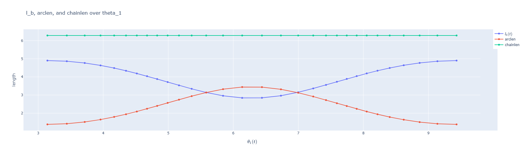
Lets verify the length of our chain is calculated correctly by plotting $l_B$, the length of the arc between $P3$ and $OF$ (the green line and the orange line from the previous plot)

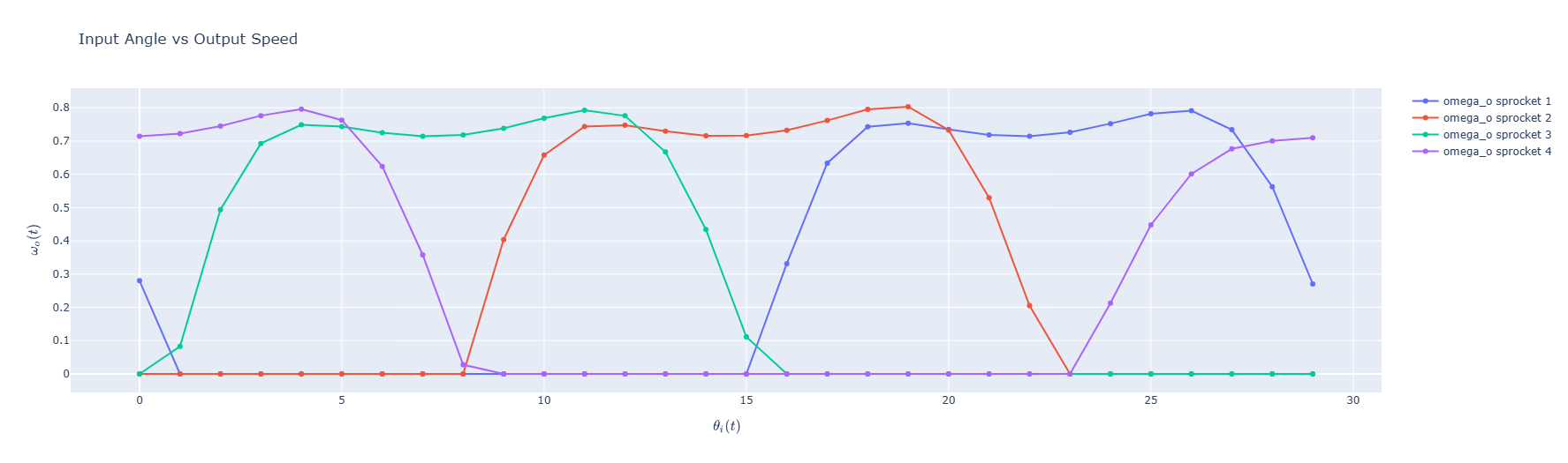
Of course we won’t use just of these systems or else we would have output torque that varies wildly resulting in a bumpy ride. What we can do is chain multiple systems together with an offset so thy take turns providing torque.

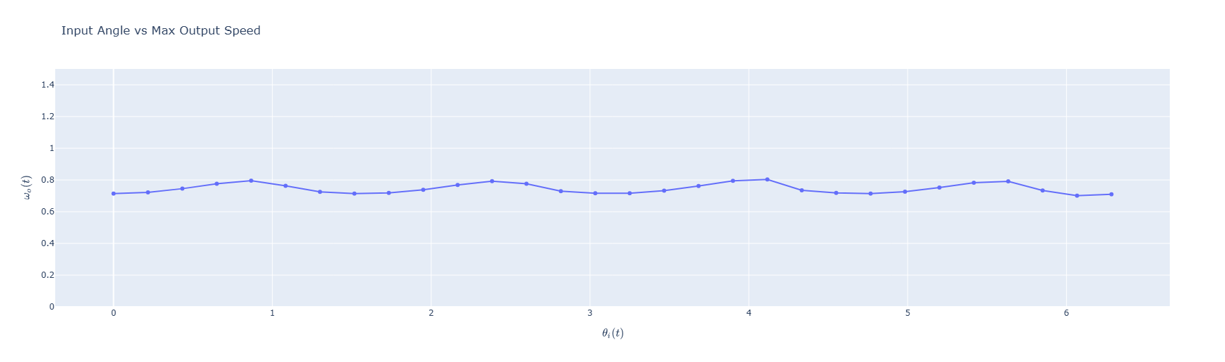
The linage with the maximum angular acceleration will be the one contributing to the whole, so we can just plot the max of the 4 systems

This line os not perfectly flat as desired, but it is much better without the elliptical input gears.

Optimization

There are different things to optimize. The first optimization is to use an elliptical gear set (yes, strange, but it seems to help) on the input drive. This was my brother, Lucas’s, idea.

I didn’t even go into optimizing the different length and positions of the linkages. Ideally, it would be optimized across the full range of the adjustable linkage ($l_A$ in our case).

Conclusion

If it wasn’t for Jason K. Moore’s excellent online book over Learn Multibody Dynamics, I don’t think I would have been able to get as fas as I did.

All of the source code can be found here. I used python for the math and took a symbolic approach the the solution. Lucas did the same thing in Matlab and took a vectorized approach.