When there is a large sum of tolerances ($n$>3), you will often see engineers doing a RSS (root sum squared) analysis of this tolerance stack to get a range that approximates the total sum of the size these these manufactured parts will fall into.

Definition

The definitions of this analysis are as follows.

$d_{g} = \sum_{i=1}^{n} a_i d_i$

$t_{wc} = \sum_{i=1}^{n} \left|a_i t_i\right|$

$t_{rss} = \sqrt{\sum_{i=1}^{n} a_n^2 t_n^2}$

and

• Minimum WC Bounds = $d_g - t_{wc}$
• Maximum WC Bounds = $d_g + t_{wc}$
• Minimum RSS Bounds = $d_g - t_{rss}$
• Maximum RSS Bounds = $d_g + t_{rss}$

where

• $n$ = the number of independent variables (dimensions) in the stackup
• $d_g$ = the mean value of the combined dimensions (or closed analysis)
• $a_i$ = sensitivity factor that defines the direction and magnitude for the ith dimension. In a one-dimensional stackup, this value is usually +1 or –1. Sometimes, in a one-dimensional stackup, this value may be +.5 or -.5 if a radius is the contributing factor for a diameter callout on a drawing.
• $d_i$ = the mean value of the ith dimension in the loop diagram.
• $t_i$ = equal bilateral tolerance of the $i$th component in the stackup.
• $t_{wc}$ = maximum expected variation (equal bilateral) using the Worst Case Model.
• $t_{rss}$ = maximum expected variation (equal bilateral) using the RSS method.

The RSS equation works for “equal $\sigma$” values. If the designer assumed that the input tolerances were ±4$\sigma$ values for the piece-part manufacturing processes, then the probability that the assembly is between ±$t_{rss}$ is 99.9937% (±4$\sigma$).

But where does RSS come from?

I understand that a “RSS Analysis” is more representative of real-life assembly results and more practical for design, but how did it come to be? I tried to consult the Dimensioning and Tolerancing Handbook by Paul J. Drake, Jr. but I could not solve it.

If we look at the Wikipedia article for adding normal distributions, we can see it defined as ^[1]

$X \sim N(\mu_X, \sigma_X^2)$

$Y \sim N(\mu_Y, \sigma_Y^2)$

$Z=X+Y,$

$Z \sim N(\mu_X + \mu_Y, \sigma_X^2 + \sigma_Y^2).$

Okay, so when two normal (aka Gaussian) distributions, X and Y, are added, the resulting mean is the sum of the two means, and the resulting variance is the sum of the two variances (variance = $\sigma^2$)

$Var(Z) = \sigma_X^2 + \sigma_Y^2$

$\sigma_Z^2 = \sigma_X^2 + \sigma_Y^2$

$9 \sigma_Z^2 = 9(\sigma_X^2 + \sigma_Y^2)$

$3\sigma_Z = \sqrt{9\sigma_X^2 + 9\sigma_Y^2}$

$3\sigma_Z = \sqrt{(3\sigma_X)^2 + (3\sigma_Y)^2}$

So if we assume the tolerance USL and LSL are ±3$\sigma$ (or any multiple really), then the sum of the tolerances is the Root Sum Squared of all the tolerances.

$t_{Z} = \sqrt{t_X^2 + t_Y^2}$

With the following assumptions

• All input tolerances are assumed to have a normal distribution
• All of the input tolerances are assumed to have equal variances
• The resulting RSS variance is equivalent to the input variances

Example

Lets say we have a motor assembly and we want to make sure that when assembled, several critical requirements are always (or almost always) met.

• Requirement 1: The gap between the shaft and the inner bearing cap must always be greater than zero to ensure that the rotor is clamped and the bearings are preloaded.
• …
• Requirement 6: The bottom of the bearing cap screw thread must never touch the bottom of the female thread on the shaft.
• …

We will focus of Requirement 6 for this example.

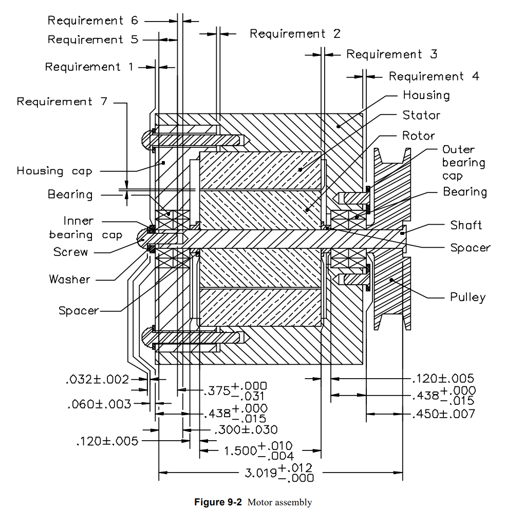
The tolerance loop for Requirement 6 looks like this:

Stack: Motor Assembly
ID Name                     Description dir  Nom.             Tol. Sens. (a) Relative Bounds 
 6    A             Screw thread length   - 0.375   + 0 / - 0.031          1  [0.344, 0.375] 
 7    B                   Washer Length   + 0.032   ± 0.002                1   [0.03, 0.034] 
 8    C Inner bearing cap turned length   +  0.06   ± 0.003                1  [0.057, 0.063] 
 9    D                  Bearing length   + 0.438   + 0 / - 0.015          1  [0.423, 0.438] 
10    E            Spacer turned length   +  0.12   ± 0.005                1  [0.115, 0.125] 
11    F                    Rotor length   +   1.5 + 0.01 / - 0.004         1   [1.496, 1.51] 
10    G            Spacer turned length   +  0.12   ± 0.005                1  [0.115, 0.125] 
 9    H                  Bearing length   + 0.438   + 0 / - 0.015          1  [0.423, 0.438] 
12    I           Pulley casting length   +  0.45   ± 0.007                1  [0.443, 0.457] 
13    J             Shaft turned length   - 3.019   + 0.012 / + 0          1  [3.019, 3.031] 
14    K               Tapped hole depth   +   0.3   ± 0.03                 1    [0.27, 0.33]

If we do a Worst Case and an RSS analysis, these are the results.

Dimension: Motor Assembly - WC Analysis - 
ID                         Name Description dir   Nom.           Tol. Sens. (a) Relative Bounds
25 Motor Assembly - WC Analysis               + 0.0615 ± 0.0955               1 [-0.034, 0.157]
37 Motor Assembly - RSS Analysis              + 0.0615 ± 0.03808              1 [0.02342, 0.09958]

If we recall the requirement, it states this stackup needed to be greater than 0. In the W.C. analysis, the bounds drop below zero, but in the RSS analysis, is does not. We can see the RSS bounds are much smaller than the Worst Case (almost 1/3 the size). If we wanted to guarantee 100% of the time, for all combinations of parts, that the requirement is met we would follow the WC analysis. The WC analysis states the requirement will not be satisfied and we need to adjust the design or clamp down on tolerances (AKA and pay more for precision). But, if we only needed the assembly to be right ~97% of the time, we can use the RSS and call it a day.

Demo created with: https://github.com/phcreery/dimstack

---

1. https://en.wikipedia.org/wiki/Sum_of_normally_distributed_random_variables ↩︎