• Introduction
• Data Massaging
  • Polynomial Fit
• Differential Geometry of a Surface Equations
  • Gauss map
  • Shape Operator
  • Mean Curvature
  • Gaussian Curvature
  • Principal Curvature
  • Radius of Curvature
  • Curvedness
  • Definitions
• Experiment
  • Setup
  • Results
  • Potential Oversights

Introduction

This entry is my attempt to understand and compute the surface curvature of a dataset for surface profile analysis. I have not taken a differential geometry class so everything here is learned in my own time by reading books, theses, and online material. I tried to test and prove everything but I cannot guarantee it is completely accurate or even correct. I will leave that up to the reader to evaluate.

I am using Python as the language of choice since it has readily available libraries for doing complex math functions and is relatively simple and popular. With that, it is by no means an optimal, fast, or portable language, but I wanted to learn and hopefully share the concept so I think it fits quite well. Having learned the concept and technique, it is quite easy to later translate the code to a faster or compiled language like C, C++, or Rust. This method of doing something once quickly and getting it working, and then doing it again another way will undoubtedly allow the programmer to come up with better techniques of implementation.

The example I used is as follows. I have a flat square sheet that has a smaller sensitive device bonded to the top it. The attached device cannot undergo a certain amount of stress or deformation due to bending or else it will fail. In this case, we are assuming perfect adhesion (or effectively ignoring the type of adhesion) but instead comparing the results with a known-good device of similar adhesion and size. If the amount of bending of the experimental device is less than the control, then we can assume it will pass. I have completed a structural model of a flat square sheet that is loaded in a complex configuration where it is experiencing forces from both the top and bottom in an irregular pattern causing the sheet to bow, fold, potato chip, and warp in a way that is difficult to calculate by hand. The device is not included in the model since we can assume the forces it exerts back onto the sheet are negligible. The model has used a tetrahedron mesh so the surface is defined as a evenly spaced triangular mesh that is not symmetric or patterned and is somewhat random. I have exported the X, Y, and Z values of the surface nodes into a CSV file for further analysis.

The rest of the document will follow this primary example along with a couple of small examples in the mix to color in relevant topics.

Data Massaging

There are many methods for smoothing out data, manipulating it to iron out inconsistencies, up-sampling, and re-meshing for better results. The one I am going I used is fitting a 2D polynomial over my dataset. This is possible since I know my data can be represented as a monge patch $f(u,v)=h$

Polynomial Fit

If we have a dataset that is an n x m matrix where the values of the matrix are the Z height of the surface and the X and Y location of those points are evenly spaced. Still, the Z values are course approximations or measurements with error, we can perform a linear least squares fitting of this two-dimensional data that not only smooths out the data but gives us a polynomial that represents the data which can be used in parametric evaluation.

The polynomial regression model: $1, x, x^2, ..., xy, x^2y, ...$ etc.

$z_i = c_0 + c_1 x_i + c_2 x_i^2 + \ldots + c_{i} y_{i} + c_{i} x_{i} y_{i} + c_i x_i^2 y_i + \ldots + c_m x_i^m y_i^m + \varepsilon_i \left( i = 1, 2, \ldots , n \right)$

can be expressed in matrix form in terms of a design matrix $\mathbf{A}$, a response vector $\vec{y}$, a parameter vector $\vec{c}$, and a vector $\vec{\varepsilon}$ of random errors. The $i$-th row of $\mathbf{A}$ and $\vec{y}$ will contain the $x$ and $y$ values for the $i$-th data sample. Then the model can be written as a system of linear equations:

$\begin{bmatrix} z_1 \\ z_2 \\ z_3 \\ \vdots \\ z_n \end{bmatrix}= \begin{bmatrix} 1 & x_1 & x_1^2 & \cdots & x_1^m y_1^m \\ 1 & x_2 & x_2^2 & \cdots & x_2^m y_2^m \\ 1 & x_3 & x_3^2 & \cdots & x_3^m y_3^m \\ \vdots & \vdots & \vdots & \ddots & \vdots \\ 1 & x_n & x_n^2 & \cdots & x_n^m y_n^m \end{bmatrix} \begin{bmatrix} c_0 \\ c_1 \\ c_2 \\ \vdots \\ c_{m^2} \end{bmatrix} + \begin{bmatrix} \varepsilon_1 \\ \varepsilon_2 \\ \varepsilon_3 \\ \vdots \\ \varepsilon_n \end{bmatrix},$

which when using pure matrix notation is written as

$\vec z = \mathbf{A} \vec c + \vec\varepsilon$

Linear least squares fitting of a two-dimensional data by christian

Differential Geometry of a Surface Equations

The differential of a parameterized surface tells us how tangent vectors on the domain get mapped to vectors in space. We can say that $df$ “pushes forward” vectors $\vec{X}$ into $\mathbb{R}^n$, yielding vectors $df(\vec{X})$

Differential

Lets say we have a parameterized surface $f$ that is defined as (with $U \subset \mathbb{R}^2$, $f:U \rightarrow \mathbb{R}^3$)

$f(u,v) := (u,v,u^2-v^2)$

the differential is simply the exterior derivative

$df = \frac{\partial f}{\partial u}du + \frac{\partial f}{\partial v}dv = (1,0,2u)du + (0,1,-2v)dv$

If we evaluate at a point in $U_{(0,0)}$

$df(U_{(0,0)}) = (1,0,2u)du + (0,1,-2v)dv = (1,0,2(0))du + (0,1,-2(0))dv = (1,1,0)$

Now lets say we want to evaluate a vector field $X$ of $U$ in $f$ (also known as a pushforward)

$X := \frac{3}{4}\frac{\partial}{\partial u} - \frac{3}{4}\frac{\partial}{\partial v}$

$df(X) = \frac{3}{4}(1,-1,2(u+v))$

and then evaluated at a point $X_{(0,0)}$

$df(X)_{(0,0)} = \frac{3}{4}(1,-1,2(u+v))_{(0,0)} = (\frac{3}{4}, -\frac{3}{4}, 0)$

--

Gauss map

A Gauss map $N$ on surface $f$ is a continuous function $n$ that assigns to each point $p \in S$ a unit normal vector $\vec{n}(p)$. ^[1]

$\vec{n}(u,v) = N(f(u,v)) = \pm \frac{\frac{\partial f}{\partial u} \times \frac{\partial f}{\partial v}}{\lVert \frac{\partial f}{\partial u} \times \frac{\partial f}{\partial v} \rVert}$

Shape Operator

The most common definition is as follows.

If $p \in M$, then for each tangent vector $\vec{v}$ to $M$ at $p$, define the shape operator: ^[2]

$S_p(\vec{v}) = - \nabla_{\vec{v}} N$

Where $N$ is a normal vector field to surface $M$ defined in a neighborhood of point $p$, and $\nabla$ is the covariant derivative. This describes the shape of the surface in the sense that we are measuring how the unit normal changes in the $\vec{v}$ direction, which describes how the tangent planes are varying in the $\vec{v}$ direction, hence describing the curving of the surface in $\mathbb{R}^3$ locally. In summary, the directional derivative on $N$ in the tangent direction $\vec{v}$ is equal to the Shape Operator at point $p$ applied to the same tangent vector $\vec{v}$

Example

Lets say we have a cylinder of radius $r$ defined as ^[3]

$x(u,v) = (r \cdot cos(u), r \cdot sin(u), v)$

then proceeding with derivation

$x_u = (-r \cdot sin(u), r \cdot cos(u), 0)$

$x_v = (0,0,1)$

$N = (cos(u), sin(u), 0)$

Then, the shape operator in $S(\vec{x_u})$ and $S(\vec{x_v})$ directions, rewritten in $\_\vec{x_u} + \_\vec{x_v}$ basis

$S(\vec{x_u}) = -N_u = (- sin(u), r \cdot cos(u), 0) = -\frac{1}{r}\vec{x_u} + 0\vec{x_v}$

$S(\vec{x_v}) = -N_v = (0, 0, 0) = 0\vec{x_u} + 0\vec{x_v}$

Thus

$S = \begin{bmatrix} -\frac{1}{r} & 0 \\ 0 & 0 \end{bmatrix}$

I find this somewhat difficult to peal apart just what this means, but Keenan Crane breaks it down and expresses it in a slightly simpler manner.

We can find the principal curvature in terms of the shape operator, which is the unique map $S: TM \rightarrow TM$ (some linear map $S$ from tangent vectors to tangent vectors) satisfying^[4]

$df(S\vec{X}) = dN(\vec{X})$

for all tangent vectors $\vec{X}$. The shape operator $S$ and the Weingarten map $dN$ essentially represent the same idea: they both tell us how the normal changes as we travel along a direction $\vec{X}$. The only difference is that $S$ specifies this change in terms of a tangent vector on $M$, whereas $dN$ gives us the change as a tangent vector in $\mathbb{R}^3$.

By a direct calculation with the matrix defining the shape operator, it can be checked that the Gaussian curvature is the determinant of the shape operator, the mean curvature is half of the trace of the shape operator, and the principal curvatures are the eigenvalues of the shape operator with their directions being the corresponding eigenvectors; moreover, the Gaussian curvature is the product of the principal curvatures and the mean curvature is their sum.

Jumping forward again to Keenan Crane's definition with $X$ a unit tangent at some point on a surface; one neat think about the principal directions and principal curvatures is that they correspond to eigenvectors and eigenvalues (respectively) of the shape operator.

$S\vec{X}_i = \kappa_i \vec{X}_i$

Example

Let's see this using an example provided by Keenan^[5]. Let's say we have a parameterized surface defined as:

$f(u,v) := (cos(u), sin(u), u+v)$

we then need to find the derivative and the Gauss Map

$df = (-sin(u), cos(u),1)du + (0,0,1)dv$

$N = (cos(u),sin(u),0)$

$dN = (-sin(u),cos(u),0)du$

from the Shape operator definition above, the function composition $f$ of $S$

$df(S\vec{X}) = dN(\vec{X})$

$df \circ S = dN$

$\begin{bmatrix} -sin(u) & 0 \\ cos(u) & 0 \\ 1 & 1 \end{bmatrix} \begin{bmatrix} S_{11} & S_{12} \\ S_{21} & S_{22} \end{bmatrix} = \begin{bmatrix} -sin(u) & 0 \\ cos(u) & 0 \\ 0 & 0 \end{bmatrix}$

solving for the shape operator $S$ we get

$S = \begin{bmatrix} 1 & 0 \\ -1 & 0 \end{bmatrix}$

the eigenvalues ($\kappa_1$, $\kappa_1$) and eigenvectors ($\vec{X}_1$, $\vec{X}_2$) are

$\kappa_1 = 0, \kappa_2 = 1, \vec{X}_1 = \begin{bmatrix} 0 \\ 1 \end{bmatrix}, \vec{X}_2 = \begin{bmatrix} -1 \\ 1 \end{bmatrix}$

if we push forward the eigenvectors from $U$ to $f$, we can find the principal directions

$df(\vec{X}_1) = (0,0,1)$

$df(\vec{X}_2) = (sin(u), -cos(u), 0)$

Now we can evaluate the principal curvatures and magnitudes for any point $(u,v)$ on the surface

We can double check our work by checking that the principal directions are orthogonal

Mean Curvature

The mean curvature at a point on a surface, p∈U, is then the average of the signed curvature over all angles θ:

$H = \frac{1}{2\pi}\int_0^{2\pi} \kappa(\theta) \;d\theta$

By applying Euler's theorem, this is equal to the average of the principal curvatures:

$H = {1 \over 2} (\kappa_1 + \kappa_2)$

For the special case of a surface defined as a function of two coordinates, e.g. $z=f(x,y)$ and using the upward pointing normal the mean curvature expression is

$H = \frac{1}{2} \frac{ \left(1 + \left(\frac{\partial f}{\partial x}\right)^2\right) \frac{\partial^2 f}{\partial y^2} - 2 \frac{\partial f}{\partial x} \frac{\partial f}{\partial y} \frac{\partial^2 f}{\partial x \partial y} + \left(1 + \left(\frac{\partial f}{\partial y}\right)^2\right) \frac{\partial^2 f}{\partial x^2} }{\left(1 + \left(\frac{\partial f}{\partial x}\right)^2 + \left(\frac{\partial f}{\partial y}\right)^2\right)^{3/2}}$

Gaussian Curvature

Gaussian curvature is defined as

$K = \kappa_1 \kappa_2$

Similarly, for a surface described as graph of a function $z=f(x,y)$, Gaussian curvature is:

$K = \frac{\frac{\partial^2 f}{\partial x^2} \cdot \frac{\partial^2 f}{\partial y^2} - \left( \frac{\partial^2 f}{\partial x \partial y} \right)^2} {\left( 1 + \left( \frac{\partial f}{\partial x} \right)^2 + \left( \frac{\partial f}{\partial x} \right)^2 \right)^2}$

Principal Curvature

Principal curvature, κ, is often defined as

$\kappa_1 = H + \sqrt{H^2 - K}$

$\kappa_2 = H - \sqrt{H^2 - K}$

With $\kappa_1$ representing the maximum and $\kappa_2$ being the minimum principal curvatures.

I think this is somewhat counter-intuitive though since the definition of $H$ and $K$ is a function of $\kappa_1$ and $\kappa_2$, but we just defined $\kappa_1$ and $\kappa_2$ as a function of $H$ and $K$ so we have a chicken or the egg situation. I prefer to find the principal curvatures first, then find the mean and gaussian curvature from them. The reason for this is the principal curvatures are not only signed scalar values, but they are vectors that point in a direction. The two equations above only give us their values but knowing both values and direction proves much more information. This is why I prefer finding the principal curvatures from the eigenvalues of the shape operator first.

Radius of Curvature

Knowing $\kappa$, the equation for the radius of curvature is

$r= \frac{1}{\kappa}$

Curvedness

It makes sense to define an always positive number $c$, henceforth referred to as the ‘curvedness’, to specify the amount, or ‘intensity’ of the surface curvature. Although several alternative definitions would serve, I chose:

$C = \sqrt{\frac{\kappa_1^2 + \kappa_2^2}{2}}$

This is similar to the RMS equation, essentially quantifying the positive valued mean curvature.

Definitions

Surfaces can be defined as either a Local Parametrization, Monge Patch, or Implicit Function. I don't find the Implicit function very useful in my case so I have skipped all references of it.

I have already given a preview of the gaussian and mean curvature defined for a monge patch. I am not going to try to derive the definitions of the first and second fundamental forms nor the shape operator, instead, I have just listed the definitions below.

Parameterized

Let $V$ be of $\mathbb{R}^2$ and $U$ be a regular surface in $\mathbb{R}^3$. Given a local parametrization f : V → U , (also shown as $f(u,v) = (x(u,v), y(u,v), z(u,v))$ where the functions $x(u,v)$, $y(u,v)$, $z(u,v)$ have continuous partial derivatives) and a unit normal vector field $n$ to $f(V)$, one defines the following objects as real-valued or matrix-valued functions on $V$.

Terminology	Notation	Definition
A unit normal vector field	$n$	$n = \pm \frac{\frac{\partial f}{\partial u} \times \frac{\partial f}{\partial v}}{\lVert \frac{\partial f}{\partial u} \times \frac{\partial f}{\partial v} \rVert}$
First fundamental form	$E$	$E=\frac{\partial f}{\partial u}\cdot\frac{\partial f}{\partial u}$
""	$F$	$F=\frac{\partial f}{\partial u}\cdot\frac{\partial f}{\partial v}$
""	$G$	$G=\frac{\partial f}{\partial v}\cdot\frac{\partial f}{\partial v}$
Second fundamental form	$L$	$L=\frac{\partial^2 f}{\partial u^2}\cdot n$
""	$M$	$M=\frac{\partial^2f}{\partial u\partial v}\cdot n$
""	$N$	$N=\frac{\partial^2f}{\partial v^2}\cdot n$
Shape operator	$P$	$P=\begin{pmatrix}L&M \\ M&N\end{pmatrix}\begin{pmatrix}E&F \\ F&G\end{pmatrix}^{-1}$
Gaussian curvature	$K$	$K=\frac{LN-M^2}{EG-F^2}$
Mean curvature	$H$	$H=\frac{GL-2FM+EN}{2(EG-F^2)}$
Principal curvatures	$\kappa_\pm$	$H\pm\sqrt{H^2-K}$

Monge Patch

The following summarizes the calculation of the above quantities relative to a Monge patch or height map $f(u, v) = (u, v, h(u, v))$ (also sometimes expressed as $z=f(x,y)$). Here $h_u$ and $h_v$ denote the two partial derivatives of $h$, with analogous notation for the second partial derivatives. The second fundamental form and all subsequent quantities are calculated relative to the given choice of unit normal vector field.

Quantity	Formula
A unit normal vector field	$n=\frac{(-h_u,-h_v,1)}{\sqrt{1+h_u^2+h_v^2}}$
First fundamental form	$\begin{pmatrix}E&F \\ F&G\end{pmatrix}=\begin{pmatrix} 1 +h_u^2 & h_u h_v \\ h_u h_v & 1 + h_v^2\end{pmatrix}$
Second fundamental form	$\begin{pmatrix}L&M \\ M&N\end{pmatrix}=\frac{1}{\sqrt{1 +h_u^2 + h_v^2}} \begin{pmatrix} h_{uu} & h_{uv} \\ h_{uv} & h_{vv} \end{pmatrix}$
Shape operator	$P=\frac{1}{(1+h_u^2+h_v^2)^{3/2}}\begin{pmatrix}h_{uu}(1+h_v^2)-h_{uv}h_uh_v&h_{uv}(1+h_u^2)-h_{uu}h_uh_v \\ h_{uv}(1+h_v^2)-h_{vv}h_uh_v&h_{vv}(1+h_u^2)-h_{uv}h_uh_v\end{pmatrix}$
Gaussian curvature	$K=\frac{h_{uu}h_{vv}-h_{uv}^2}{(1+h_u^2+h_v^2)^2}$
Mean curvature	$H=\frac{(1+h_v^2)h_{uu}-2h_uh_vh_{uv}+(1+h_u^2)h_{vv}}{2(1+h_u^2+h_v^2)^{3/2}}$

Experiment

Setup

Lets say we have a complex loaded sheet that is being compressed from behind and a fragile part attached to it. Under these loading conditions, we know the device does not fail. This will be our control. Now, we want to know if a larger device fixed to it will be able to perform without failing due to stress.

I will be using COMSOL to simulate deformation of the surface which we will use os the dataset for the theory. I will also simulate the stress of the part which will serve as the results to compare the theory to.

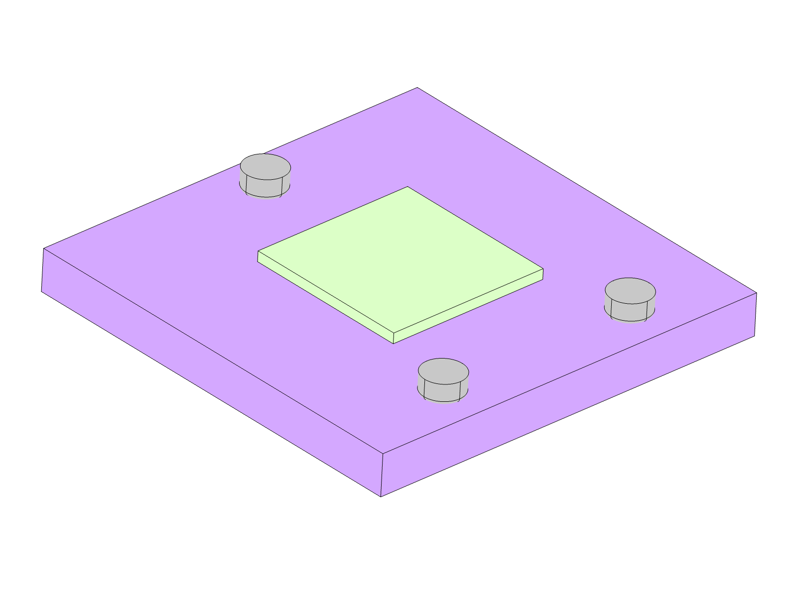Setup 1. Module (Green), Carrier (Purple), Support (Grey)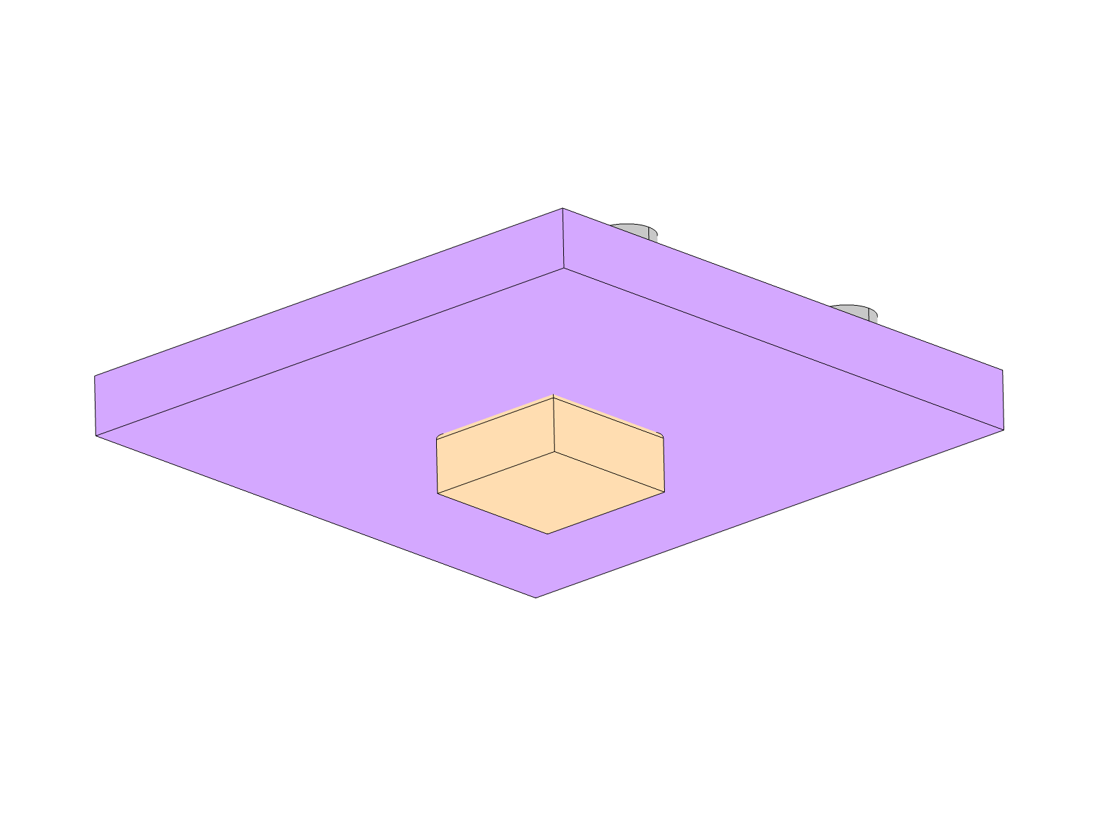Setup 1 back-side. Load (Orange)

The initial setup has an 8x8x0.5 $mm$ Silicon Module adhered to the center of the top-side of the carrier.

Setup 1 in COMSOL

For the next setup, 2, I simply doubled the load to 40 $N/mm^2$ For setup 3, I increased the carrier thickness from 2 to 3 $mm$.

Setup 3 in COMSOL

For setup 4, I went back to 2 $mm$ thick carrier and I used 4 support members in the corners separated 16mm apart.

Setup 4 in COMSOL

For setup 5, I increased the module size from 8x8 $mm$ to 10x10 $mm$. For setup 6, I went back to the triangular loading, keeping the 40 $N/mm^2$ load and 10x10 $mm$ module. For setup 7, I kept the larger module and bumped the load back down to 20 $N/mm^2$

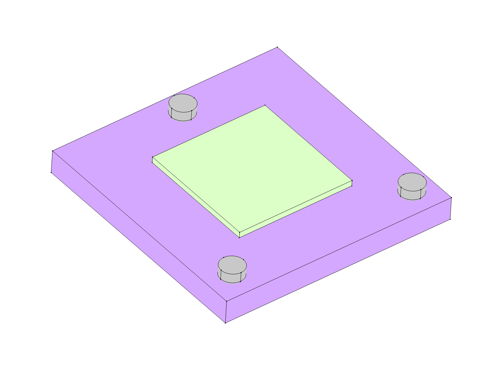Setup 7

Results

After the models were setup in FEA, I exported the Max Stress and the Deformation of the mesh in the Module Attach region as X,Y,X pairs in a text file.

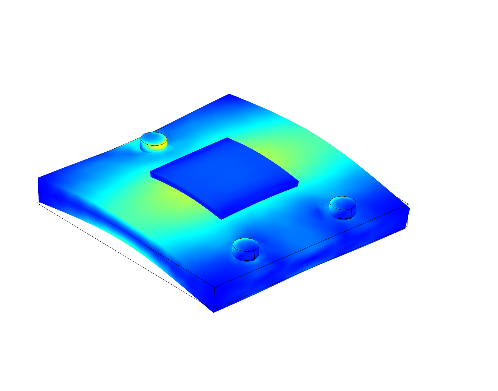
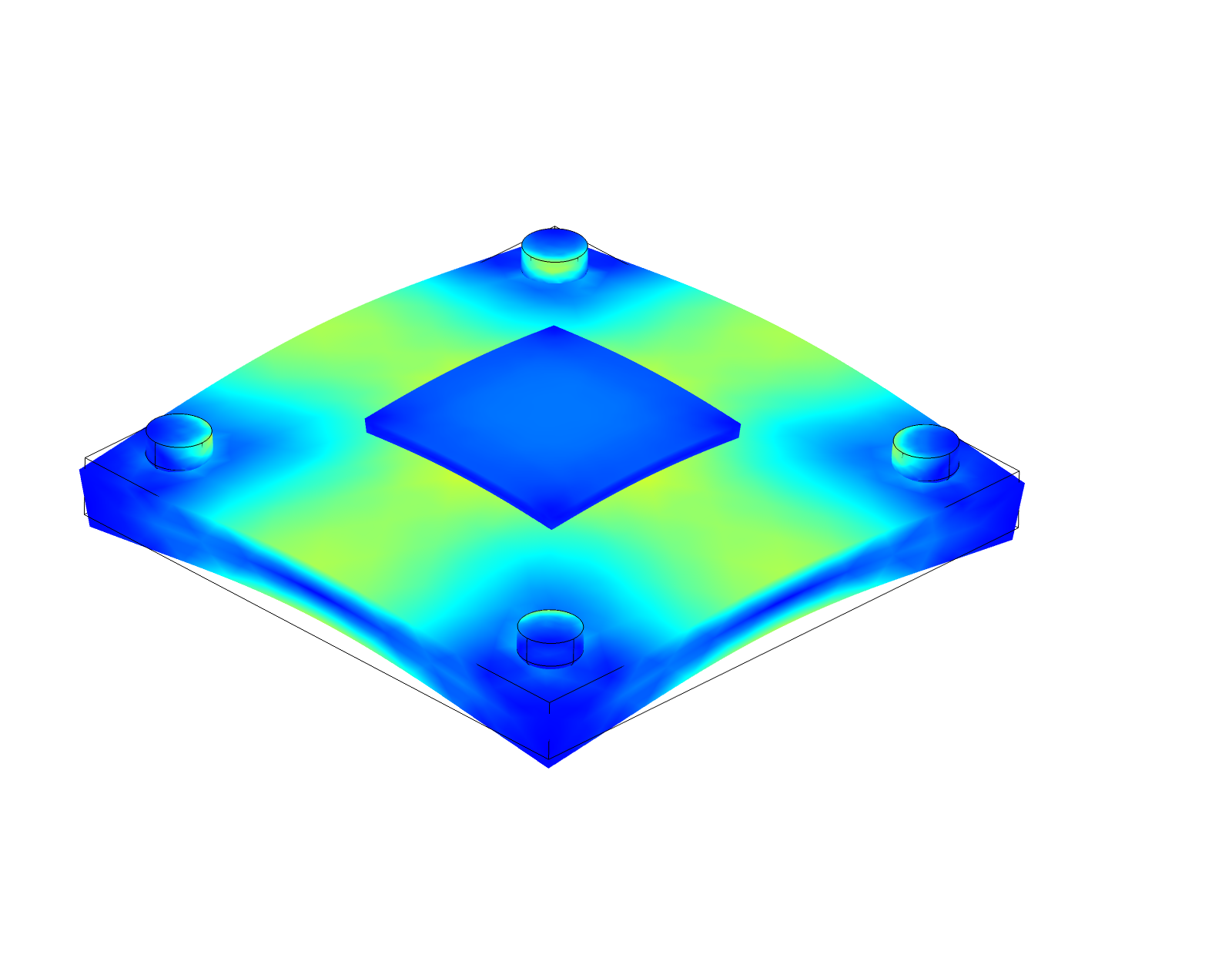
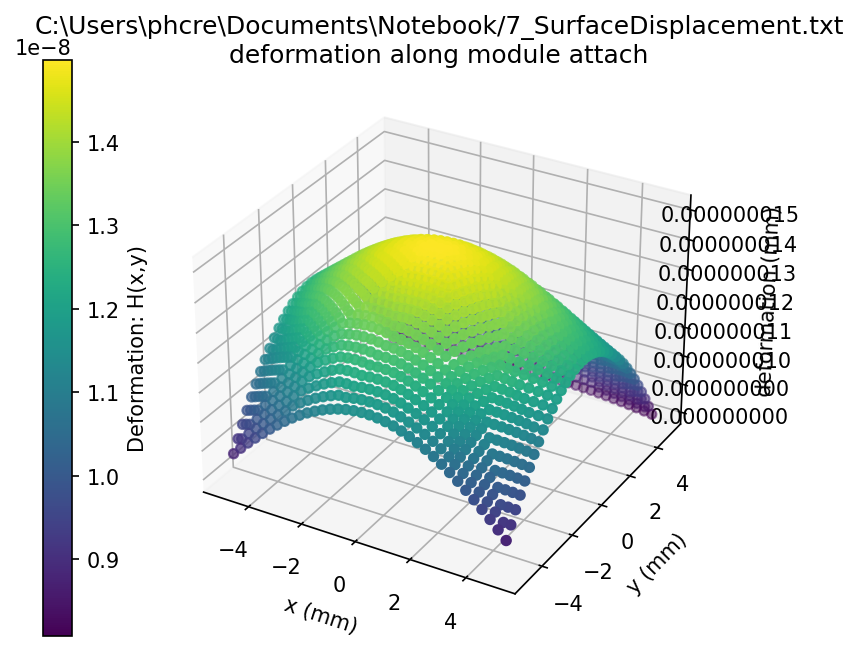Setup 7 Deformation

I then fed this into a python notebook to compute maximum curvedness.

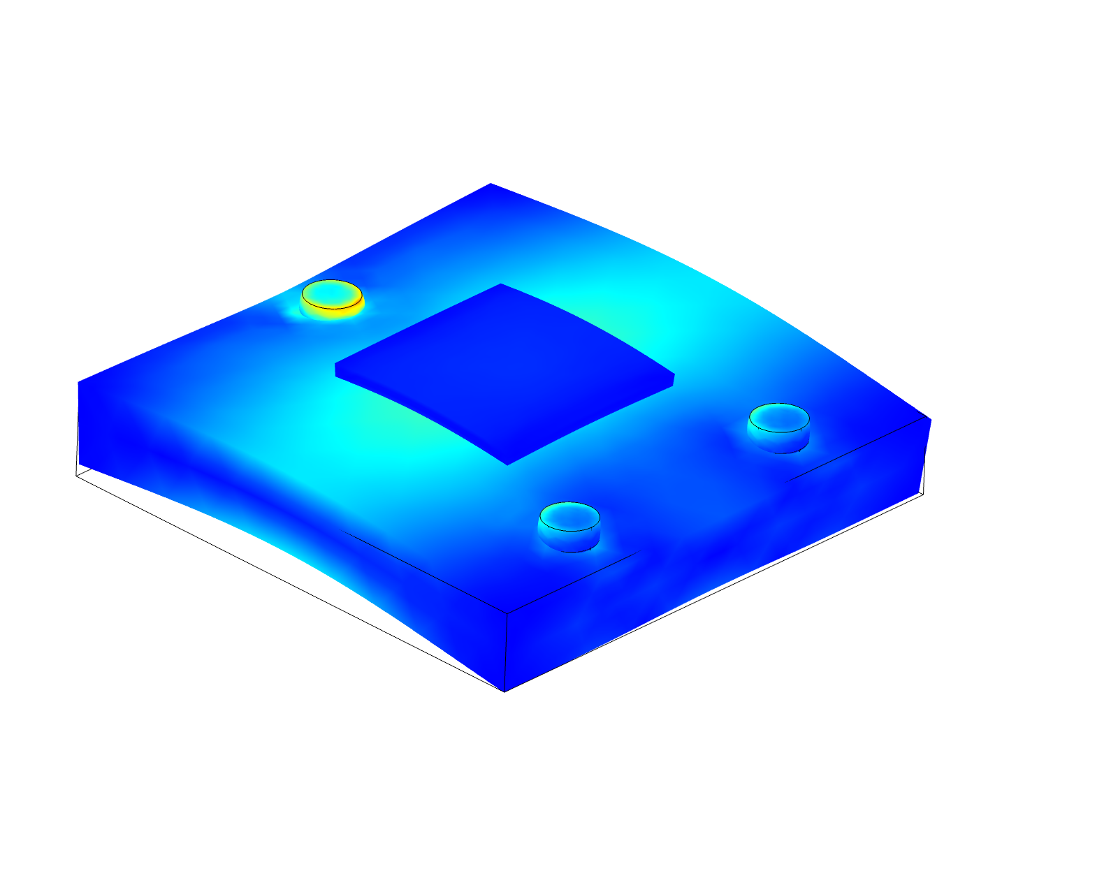
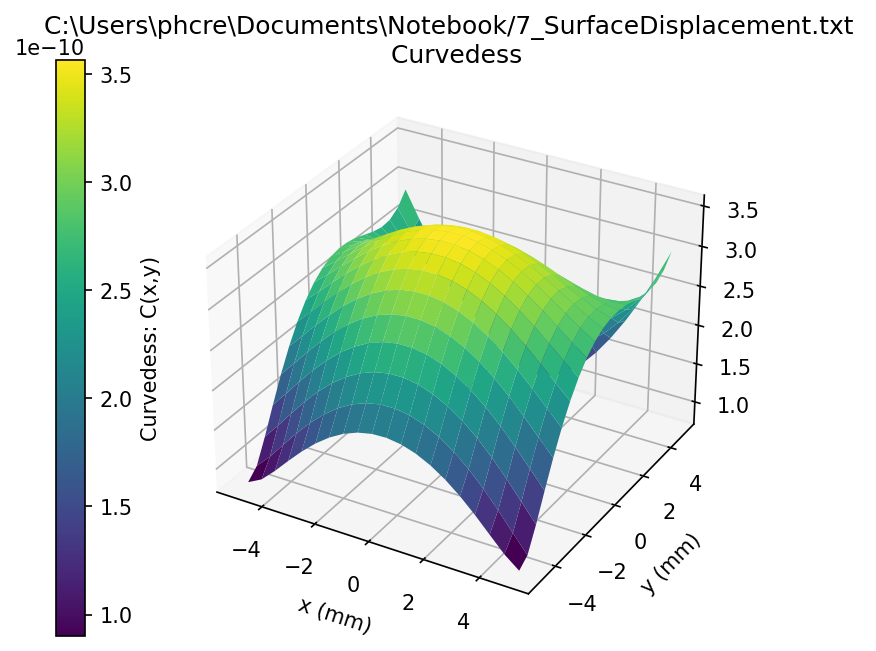Setup 7 Curvedness

If we run the larger device under a parametric sweep of different load, thickness, and support structure, we should be able to plot the amount of curvature in relation to the stress in different loading setups.

Setup	Load	Support Configuration	Device Size	Carrier Thickness	Max Stress of Module	Max Curvedness
	N/m^2		mm	mm	N/m^2	1/m
1	20	-5/5 Triangle	8x8	2	23.47	3.62E-10
2	40	-5/5 Triangle	8x8	2	55.34	7.14E-10
3	40	-5/5 Triangle	8x8	3	18.69	2.52E-10
4	40	-8/8 Corners	8x8	2	55.08	7.96E-10
5	40	-8/8 Corners	10x10	2	61.9	7.52E-10
6	40	-5/5 Triangle	10x10	2	60.84	6.98E-10
7	20	-5/5 Triangle	10x10	2	30.36	3.58E-10

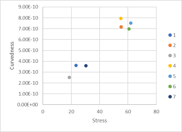Max Stress vs Max Cuvedness

From this dataset, we can see there is a small correlation between the measured surface curvature of the device and the resulting stress in the module. In a sense, it it almost like a stress strain graph of complex geometry.

Potential Oversights

All of these experiments were done with several uniform parameters. Any one of these could change the results but I kept them constant for simplicity.

Parameter	Value	Examples
Module Geometry	Rectangular cuboid of uniform thickness	Rectangular prism, etc.
Carrier Geometry	Rectangular cuboid of uniform thickness	Complex shape
Load Geometry	5x5 mm square load placed in the center of the backside of the carrier	Different sized, placed in a different location, etc.
Support Configuration	3 pads that the carrier presses up against.
Materials	I used generic material for this study but kept them the same across the experiments.	If I change them, the results may vary

I am also aware the COMSOL is able to calculate the surface curvature but not all FEA software will do this. Plus, most of this exercise was because I wanted to see if I could calculate it myself. I am interested in seeing if I could compare my curvature calculations to that of the COMSOL.

---

1. https://e.math.cornell.edu/people/belk/differentialgeometry/Outline - The Gauss Map.pdf ↩︎

2. https://jhavaldar.github.io/assets/2017-07-16-diffgeo-notes5.pdf ↩︎

3. https://www.appstate.edu/~greenwaldsj/class/4140/shapeoperator.pdf ↩︎

4. http://wordpress.discretization.de/geometryprocessingandapplicationsws19/a-quick-and-dirty-introduction-to-the-curvature-of-surfaces/ ↩︎

5. https://brickisland.net/DDGFall2017/wp-content/uploads/2017/10/CMU_DDG_Fall2017_08_Surfaces.pdf ↩︎